Stability analysis of a softening gradient damage model

Authors:

• Jack S. Hale (University of Luxembourg)

• Corrado Maurini (Sorbonne Université)

In this notebook we implement a stability analysis on a selective linear-softening (S-LS) gradient damage model. For a full overview of the theoretical aspects of the damage model we refer the reader to:

• Stability and crack nucleation in variational phase-field models of fracture: effects of length-scales and stress multi-axiality. Zolesi and Maurini 2024. Preprint. https://hal.sorbonne-universite.fr/hal-04552309

and for the numerical stability analysis to:

• Numerical bifurcation and stability analysis of variational gradient-damage models for phase-field fracture, León Baldelli and Maurini, Journal of the Mechanics and Physics of Solids, 2021. https://hal.science/hal-03106368v2

The essence of the approach is as follows:

1. We define a S-LS gradient damage model via its energy functional \(\mathcal{E}\) with a split of the elastic energy into deviatoric and spherical parts, with each associated with a selective softening parameter.

2. Following the previous tutorial, we solve for the problem state \((u_t, \alpha_t)\) in pseudo-time \(t\) using the alternate minimisation algorithm with a pointwise bound constraint to ensure irreversibility.

3. To understand the stability of the equilibrium state we then solve an eigenvalue problem associated with the second-order state stability condition. An stationary state \((u_t, \alpha_t)\) is said to be incrementally stable if the reduced Hessian of the energy is positive:

   \[ \mathcal{E}^{''}(u, \alpha)(v, \beta) > 0, \quad \forall (v, \beta) \in \mathcal{N}_0, \]

   where \(\mathcal{N}_0\) is the space of admissable displacements and damages where the constraints are not strongly active.

The numerical aspects of solving this problem will be discussed below.

Preamble

We begin by importing the required Python modules.

Here we use will use the restriction functionality of dolfiny.

You can install dolfiny in your container by opening a shell and running:

pip install git+https://github.com/fenics-dolfiny/dolfiny.git@v0.9.0

import sys

from mpi4py import MPI
from petsc4py import PETSc

import numpy as np
from dolfiny.restriction import Restriction
from slepc4py import SLEPc

import basix
import basix.ufl
import dolfinx
import dolfinx.fem as fem
import dolfinx.fem.petsc
import dolfinx.la as la
import dolfinx.plot as plot
import ufl

sys.path.append("../utils/")

import matplotlib.pyplot as plt
from inactive_set import inactive_damage_dofs
from meshes import generate_bar_mesh
from petsc_problems import SNESProblem
from plots import plot_damage_state
from pyvista.utilities.xvfb import start_xvfb

start_xvfb(wait=0.5)

Mesh

We define the mesh using a provided function which uses gmsh internally. This function returns the mesh and so-called mesh tags mt and facet tags ft that allow us to integrate over, or apply boundary conditions to, specific parts of the boundary. The dictionaries mm and fm contain a map between easy-to-remember strings and numbers in the tags mt and ft, respectively.

Lx = 1.0  # Size of domain in x-direction
Ly = 0.1  # Size of domain in y-direction
ell = 0.5  # Regularisation length scale.

comm = MPI.COMM_WORLD
msh, mt, ft, mm, fm = generate_bar_mesh(comm, Lx=Lx, Ly=Ly, lc=ell / 40.0)

import pyvista  # noqa: E402

pyvista.start_xvfb(wait=0.1)
pyvista.set_jupyter_backend("static")

vtk_mesh = plot.vtk_mesh(msh)
grid = pyvista.UnstructuredGrid(*vtk_mesh)
plotter = pyvista.Plotter()
plotter.add_mesh(grid, show_edges=True)
plotter.camera_position = "xy"
if not pyvista.OFF_SCREEN:
    plotter.show()

Info    : Optimizing mesh (Netgen)...
Info    : Done optimizing mesh (Wall 1.893e-06s, CPU 3e-06s)
Info    : Meshing 1D...
Info    : [  0%] Meshing curve 1 (Line)
Info    : [ 30%] Meshing curve 2 (Line)
Info    : [ 60%] Meshing curve 3 (Line)
Info    : [ 80%] Meshing curve 4 (Line)
Info    : Done meshing 1D (Wall 0.000492209s, CPU 0.000564s)
Info    : Meshing 2D...
Info    : Meshing surface 1 (Plane, Delaunay)
Info    : Done meshing 2D (Wall 0.0146949s, CPU 0.014664s)
Info    : 906 nodes 1814 elements

Setting the stage

We setup the finite element space, the states, the bound constraints on the states and UFL measures.

We use (vector-valued) linear Lagrange finite elements on triangles for displacement and damage.

element_u = basix.ufl.element("Lagrange", msh.basix_cell(), degree=1, shape=(msh.geometry.dim,))
V_u = fem.functionspace(msh, element_u)

element_alpha = basix.ufl.element("Lagrange", msh.basix_cell(), degree=1)
V_alpha = fem.functionspace(msh, element_alpha)

u = fem.Function(V_u, name="displacement")
alpha = fem.Function(V_alpha, name="damage")

alpha_lb = dolfinx.fem.Function(V_alpha, name="lower bound")
alpha_ub = dolfinx.fem.Function(V_alpha, name="upper bound")
alpha_ub.x.array[:] = 1.0

dx = ufl.Measure("dx", domain=msh)
ds = ufl.Measure("ds", domain=msh, subdomain_data=ft)

Boundary conditions

We impose Dirichlet boundary conditions on components of the displacement and the damage field on the appropriate parts of the boundary.

In the previous example we use predicates to locate the facets on the boundary. An alternative approach is to directly use the facet tags fm returned directly by the mesh generator. This can be helpful when dealing with applying boundary conditions on meshes with complex curved surfaces.

bc_dofs_ux_left = dolfinx.fem.locate_dofs_topological(
    V_u.sub(0), msh.topology.dim - 1, ft.find(fm["left"])
)

bc_dofs_ux_right = dolfinx.fem.locate_dofs_topological(
    V_u.sub(0), msh.topology.dim - 1, ft.find(fm["right"])
)

bc_dofs_uy_bottom = dolfinx.fem.locate_dofs_topological(
    V_u.sub(1), msh.topology.dim - 1, ft.find(fm["bottom"])
)

u_D = fem.Constant(msh, 0.0)
bcs_u = [
    fem.dirichletbc(0.0, bc_dofs_ux_left, V_u.sub(0)),
    fem.dirichletbc(0.0, bc_dofs_uy_bottom, V_u.sub(1)),
    fem.dirichletbc(u_D, bc_dofs_ux_right, V_u.sub(0)),
]
bc_dofs_u_all = np.concatenate([bc_dofs_ux_left, bc_dofs_uy_bottom, bc_dofs_ux_right])

bc_dofs_alpha_left = dolfinx.fem.locate_dofs_topological(
    V_alpha, msh.topology.dim - 1, ft.find(fm["left"])
)

bc_dofs_alpha_right = dolfinx.fem.locate_dofs_topological(
    V_alpha, msh.topology.dim - 1, ft.find(fm["right"])
)

# Case 1: Dirichlet condition on left and right ends
bcs_alpha = [
    fem.dirichletbc(0.0, bc_dofs_alpha_left, V_alpha),
    fem.dirichletbc(0.0, bc_dofs_alpha_right, V_alpha),
]
bc_dofs_alpha_all = np.concatenate([bc_dofs_alpha_left, bc_dofs_alpha_right])

Variational formulation of the problem

Selective Linear-Softening model

We will now define the free S-LS parameters and some derived ones necessary for the analysis. The descriptions are made inline with comments for readability.

# Additional parameters
nu_0 = 0.3  # Poisson's ratio.

# Define free parameters for SL-S model. Table 1 Zelosi and Maurini, third row.
E_0 = 1.0  # Young's modulus
G_c = 1.0  # Fracture toughness
sigma_peak = 1.0  # Peak strength
ell = 0.5  # Regularisation length scale (repeated)

# Derived quantities from four free parameters
mu_0 = E_0 / (2.0 * (1.0 + nu_0))  # First Lame parameter of undamaged material
kappa_0 = E_0 / (2.0 * (1 - nu_0))  # Bulk modulus of undamaged material
w_1 = G_c / (np.pi * ell)  # Energy required to damage unit volume in a homogeneous process

# Softening parameters for spherical and deviatoric contributions
gamma = gamma_mu = gamma_kappa = (2 * G_c * E_0) / (np.pi * ell * sigma_peak**2)
t_peak = sigma_peak / E_0  # Peak strain
t_star = 2 * G_c / (sigma_peak * Lx)  # Final failure strain for homogeneous solution
t_f = 2 * G_c / (sigma_peak * np.pi * ell)  # Final failure strain for localised solution
ell_ch = gamma * np.pi * ell  # Cohesive zone length scale.

# Dimensionless parameters. The model response depends on these two parameters
# only.
lmbda_str = Lx / ell_ch  # Structural length
lmbda_reg = ell / ell_ch  # Regularisation length

We print a summary of the important variables.

print(f"lmbda_str: {lmbda_str}")
print(f"lmbda_reg: {lmbda_reg}")
print(f"t_peak: {t_peak}")

lmbda_str: 0.5
lmbda_reg: 0.25
t_peak: 1.0

The strain energy density of the S-LS constitutive model can be written as

\[ \mathcal{E}(u, \alpha) = \frac{\kappa(\alpha)}{2} [\mathrm{tr}(\varepsilon)]^2 + \mu(\alpha) | \mathrm{dev}(\varepsilon) |^2 + w_1(w(\alpha) + \ell^2 | \nabla \alpha | ^ 2), \]

where \(\varepsilon\) is the usual small strain tensor as a function of the displacements \(u\), \(\mathrm{tr}\) is the trace operator, \(\mathrm{dev}\) takes the deviatoric part of a tensor, and \(\alpha\) is the damage field. Here we do not consider any distinction of the elastic energy in positive and negative part, focusing on the case of traction-like loading.

The dissipation function is

\[ w(\alpha) := 1 - (1 - \alpha)^2, \]

and spherical and deviatoric degradation functions are

\[ \kappa(\alpha) := \frac{1 - w(\alpha)}{1 + (\gamma_{\kappa} - 1) w (\alpha)} \kappa_0, \]

\[ \mu(\alpha) := \frac{1 - w(\alpha)}{1 + (\gamma_{\mu} - 1) w (\alpha)} \mu_0. \]

Note that in this example we set \(\gamma_\kappa = \gamma_\mu\), i.e. we do not selectively soften.

def eps(u):
    return ufl.sym(ufl.grad(u))


def w(alpha):
    return 1.0 - (1.0 - alpha) ** 2


def mu(alpha):
    return mu_0 * (1.0 - w(alpha)) / (1.0 + (gamma_mu - 1.0) * w(alpha))


def kappa(alpha):
    return kappa_0 * (1.0 - w(alpha)) / (1.0 + (gamma_kappa - 1.0) * w(alpha))


def dissipation_energy_density(alpha):
    w_1_ = dolfinx.fem.Constant(msh, w_1)
    ell_squared = dolfinx.fem.Constant(msh, ell * ell)
    return w_1_ * (w(alpha) + ell_squared * ufl.inner(ufl.grad(alpha), ufl.grad(alpha)))


def deviatoric_energy_density(eps, alpha):
    return mu(alpha) * ufl.inner(ufl.dev(eps), ufl.dev(eps))


def isotropic_energy_density(eps, alpha):
    return 0.5 * kappa(alpha) * ufl.tr(eps) * ufl.tr(eps)


def elastic_energy_density(eps, alpha):
    return deviatoric_energy_density(eps, alpha) + isotropic_energy_density(eps, alpha)


def total_energy(u, alpha):
    return elastic_energy_density(eps(u), alpha) * dx + dissipation_energy_density(alpha) * dx


def sigma(eps, alpha):
    eps_ = ufl.variable(eps)
    sigma = ufl.diff(elastic_energy_density(eps_, alpha), eps_)
    return sigma


energy = total_energy(u, alpha)

Numerical solution for equilibrium

We will use the same alternate minimisation algorithm as in the previous notebook to solve at each pseudo-time step. We do not repeat the details here.

E_u = ufl.derivative(energy, u, ufl.TestFunction(V_u))
E_u_u = ufl.derivative(E_u, u, ufl.TrialFunction(V_u))
elastic_problem = SNESProblem(E_u, u, bcs_u, J=E_u_u)

b_u = la.create_petsc_vector(V_u.dofmap.index_map, V_u.dofmap.index_map_bs)
J_u = dolfinx.fem.petsc.create_matrix(elastic_problem.a)

b_u = la.create_petsc_vector(V_u.dofmap.index_map, V_u.dofmap.index_map_bs)
J_u = dolfinx.fem.petsc.create_matrix(elastic_problem.a)

# Setup linear elasticity problem and solve
solver_u_snes = PETSc.SNES().create()
solver_u_snes.setOptionsPrefix("elasticity_")
solver_u_snes.setFunction(elastic_problem.F, b_u)
solver_u_snes.setJacobian(elastic_problem.J, J_u)

opts = PETSc.Options()
opts["elasticity_snes_type"] = "ksponly"
opts["elasticity_ksp_type"] = "preonly"
opts["elasticity_pc_type"] = "lu"
opts["elasticity_pc_factor_mat_solver_type"] = "mumps"
opts["elasticity_snes_rtol"] = 1.0e-8
opts["elasticity_snes_atol"] = 1.0e-8
solver_u_snes.setFromOptions()

# Setup damage problem.
E_alpha = ufl.derivative(energy, alpha, ufl.TestFunction(V_alpha))
E_alpha_alpha = ufl.derivative(E_alpha, alpha, ufl.TrialFunction(V_alpha))

damage_problem = SNESProblem(E_alpha, alpha, bcs_alpha, J=E_alpha_alpha)

b_alpha = la.create_petsc_vector(V_alpha.dofmap.index_map, V_alpha.dofmap.index_map_bs)
J_alpha = fem.petsc.create_matrix(damage_problem.a)

# Create Newton variational inequality solver and solve
solver_alpha_snes = PETSc.SNES().create()
solver_alpha_snes.setOptionsPrefix("damage_")
solver_alpha_snes.setFunction(damage_problem.F, b_alpha)
solver_alpha_snes.setJacobian(damage_problem.J, J_alpha)
solver_alpha_snes.setVariableBounds(alpha_lb.x.petsc_vec, alpha_ub.x.petsc_vec)

opts["damage_snes_type"] = "vinewtonrsls"
opts["damage_ksp_type"] = "preonly"
opts["damage_pc_type"] = "lu"
opts["damage_pc_factor_mat_solver_type"] = "mumps"
opts["damage_snes_rtol"] = 1.0e-8
opts["damage_snes_atol"] = 1.0e-8
opts["damage_snes_max_it"] = 50

solver_alpha_snes.setFromOptions()


def simple_monitor(u, alpha, iteration, error_L2):
    pass


def alternate_minimization(u, alpha, atol=1e-6, max_iter=100, monitor=simple_monitor):
    alpha_old = fem.Function(alpha.function_space)
    alpha_old.x.array[:] = alpha.x.array

    for iteration in range(max_iter):
        # Solve displacement
        solver_u_snes.solve(None, u.x.petsc_vec)
        # This forward scatter is necessary when `solver_u_snes` is of type `ksponly`.
        u.x.scatter_forward()

        # Solve damage
        solver_alpha_snes.solve(None, alpha.x.petsc_vec)

        # check error and update
        L2_error = ufl.inner(alpha - alpha_old, alpha - alpha_old) * dx
        error_L2 = np.sqrt(comm.allreduce(fem.assemble_scalar(fem.form(L2_error)), op=MPI.SUM))
        alpha_old.x.array[:] = alpha.x.array

        if monitor is not None:
            monitor(u, alpha, iteration, error_L2)

        if error_L2 <= atol:
            return (error_L2, iteration)

    raise RuntimeError(f"Could not converge after {max_iter} iterations, error {error_L2:3.4e}")

Numerical solution for stability

DOLFINx has support for assembling block structured matrices and vectors into PETSc block structured linear algebra objects. This allows us to compose the full residual and full Jacobian (Hessian) on from its sub-components.

\[\begin{split} F = \begin{bmatrix} F_u \\ F_{\alpha} \end{bmatrix} \end{split}\]

\[\begin{split} A = \begin{bmatrix} A_{uu} && A_{u \alpha} \\ A_{\alpha u} && A_{\alpha \alpha} \end{bmatrix} \end{split}\]

\[\begin{split} B = \begin{bmatrix} B_{uu} && 0 \\ 0 && B_{\alpha\alpha} \end{bmatrix} \end{split}\]

# Block residual
F = [None for i in range(2)]
F[0] = ufl.derivative(energy, u, ufl.TestFunction(V_u))
F[1] = ufl.derivative(energy, alpha, ufl.TestFunction(V_alpha))

# Block A
A = [[None for i in range(2)] for j in range(2)]
A[0][0] = ufl.derivative(F[0], u, ufl.TrialFunction(V_u))
A[0][1] = ufl.derivative(F[0], alpha, ufl.TrialFunction(V_alpha))
A[1][0] = ufl.derivative(F[1], u, ufl.TrialFunction(V_u))
A[1][1] = ufl.derivative(F[1], alpha, ufl.TrialFunction(V_alpha))

# Block B
B = [[None for i in range(2)] for j in range(2)]
B[0][0] = ufl.inner(ufl.TrialFunction(V_u), ufl.TestFunction(V_u)) * dx
B[1][1] = ufl.inner(ufl.TrialFunction(V_alpha), ufl.TestFunction(V_alpha)) * dx

A_form = fem.form(A)
B_form = fem.form(B)

A = fem.petsc.create_matrix_block(A_form)
B = fem.petsc.create_matrix_block(B_form)

SLEPc is a package for solving large-scale sparse eigenvalue problems. Here we use a Krylov-Schur algorithm with shift-and-invert (sinvert) to accelerate the convergence of the spectrum to the eigenvalues around -0.1. This shift-and-invert acceleration involves the solution of a linear system which we again perform with LU decomposition.

stability_solver = SLEPc.EPS().create()
stability_solver.setOptionsPrefix("stability_")

opts["stability_eps_type"] = "krylovschur"
opts["stability_eps_target"] = "smallest_real"
opts["stability_eps_target"] = -0.1
opts["stability_st_type"] = "sinvert"
opts["stability_st_shift"] = -0.1
opts["stability_eps_tol"] = 1e-7
opts["stability_st_ksp_type"] = "preonly"
opts["stability_st_pc_type"] = "lu"
opts["stability_st_pc_factor_mat_solver_type"] = "mumps"
opts["stability_st_mat_mumps_icntl_24"] = 1
stability_solver.setFromOptions()

ts = np.linspace(0.0, 2.3 * t_peak, 30)

# Array to store results
energies = np.zeros((ts.shape[0], 3))
eigenvalues = np.zeros((ts.shape[0], 2))
forces = np.zeros((ts.shape[0], 1))

Now we begin the pseudo-time stepping loop. We first solve for the stationary state using alternate minimisation. We then assemble the Hessian and the mass matrix on the entire space, before restricting it to the space \(\mathcal{N}_0\) of not-strongly-active constraints. This is done at the linear algebra level by:

1. Finding the inactive set for the displacements \(u\). As there is no bound constraint on \(u\) this is all of the degrees of freedom associated with \(u\).

2. Removing from the set produced in 1. all degrees of freedom associated with the Dirichlet boundary conditions on \(u\).

3. Finding the inactive set for the damage \(\alpha\). Note that PETSc contains a method for finding this set, but it does not currently appear to be working, so we have written a method inactive_damage_dofs that finds this set according to the definition for \(\mathcal{I}(x)\) found in the previous notebook.

4. Removing from the set produced in 3. all degrees of freedom associated with Dirichlet boundary conditions on \(\alpha\).

We then use the Restriction class from dolfiny to take the matrices on the full space and keep only the rows and columns associated with the sets of degrees of freedom defined in 2. and 4.

elastic_energy_form = dolfinx.fem.form(elastic_energy_density(eps(u), alpha) * dx)
dissipation_energy_form = dolfinx.fem.form(dissipation_energy_density(alpha) * dx)
force_form = dolfinx.fem.form(sigma(eps(u), alpha)[0, 0] * ds(fm["right"]))

u.x.array[:] = 0.0
alpha.x.array[:] = 0.0

for i_t, t in enumerate(ts):
    u_D.value = energies[i_t, 0] = eigenvalues[i_t, 0] = t

    print(f"-- Solving for load = {t:3.2f} --")

    # Update the lower bound to ensure irreversibility of damage field.
    alpha_lb.x.array[:] = alpha.x.array
    alpha_lb.x.scatter_forward()
    alternate_minimization(u, alpha)
    plot_damage_state(u, alpha, load=t)

    # Assemble operators on the entire space, then restrict.
    A.zeroEntries()
    fem.petsc.assemble_matrix_block(A, A_form)
    A.assemble()

    B.zeroEntries()
    fem.petsc.assemble_matrix_block(B, B_form)
    B.assemble()

    # Construct inactive set on displacement.
    u_inactive_set = np.arange(
        0, V_u.dofmap.index_map_bs * V_u.dofmap.index_map.size_local, dtype=np.int32
    )
    u_restrict = np.setdiff1d(u_inactive_set, bc_dofs_u_all)

    # Construct inactive set on damage.
    alpha_restrict = inactive_damage_dofs(alpha, alpha_lb, b_alpha, bc_dofs_alpha_all)

    restriction = Restriction([V_u, V_alpha], [u_restrict, alpha_restrict])

    # Create restricted operators.
    A_restricted = restriction.restrict_matrix(A)
    B_restricted = restriction.restrict_matrix(B)

    stability_solver.setOperators(A_restricted, B_restricted)
    stability_solver.solve()

    num_converged = stability_solver.getConverged()
    assert num_converged > 1

    # Store first eigenvalue
    eigenvalues[i_t, 1] = stability_solver.getEigenvalue(0).real

    # Calculate the energies
    energies[i_t, 1] = comm.allreduce(
        dolfinx.fem.assemble_scalar(elastic_energy_form),
        op=MPI.SUM,
    )
    energies[i_t, 2] = comm.allreduce(
        dolfinx.fem.assemble_scalar(dissipation_energy_form),
        op=MPI.SUM,
    )

    # Calculate the global force
    forces[i_t] = comm.allreduce(
        dolfinx.fem.assemble_scalar(force_form),
        op=MPI.SUM,
    )

-- Solving for load = 0.00 --

-- Solving for load = 0.08 --
-- Solving for load = 0.16 --
-- Solving for load = 0.24 --
-- Solving for load = 0.32 --
-- Solving for load = 0.40 --
-- Solving for load = 0.48 --
-- Solving for load = 0.56 --

-- Solving for load = 0.63 --
-- Solving for load = 0.71 --
-- Solving for load = 0.79 --
-- Solving for load = 0.87 --
-- Solving for load = 0.95 --
-- Solving for load = 1.03 --

-- Solving for load = 1.11 --
-- Solving for load = 1.19 --

-- Solving for load = 1.27 --
-- Solving for load = 1.35 --

-- Solving for load = 1.43 --

-- Solving for load = 1.51 --

-- Solving for load = 1.59 --

-- Solving for load = 1.67 --

-- Solving for load = 1.74 --

-- Solving for load = 1.82 --

-- Solving for load = 1.90 --

-- Solving for load = 1.98 --

-- Solving for load = 2.06 --

-- Solving for load = 2.14 --

-- Solving for load = 2.22 --

-- Solving for load = 2.30 --

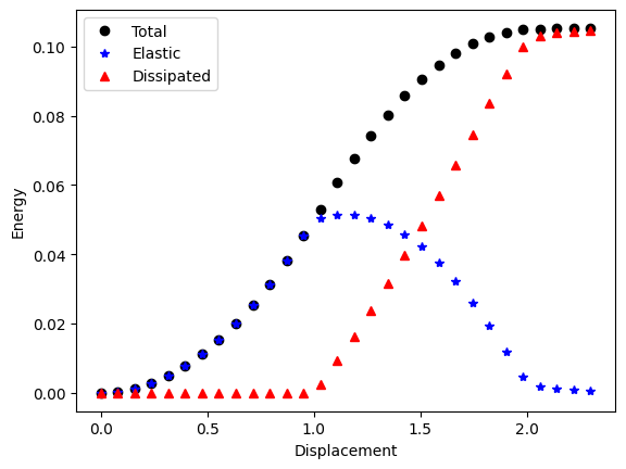
Verification

Let’s check the total, elastic and dissipated energies visually.

(p3,) = plt.plot(energies[:, 0], energies[:, 1] + energies[:, 2], "ko", linewidth=2, label="Total")
(p1,) = plt.plot(energies[:, 0], energies[:, 1], "b*", linewidth=2, label="Elastic")
(p2,) = plt.plot(energies[:, 0], energies[:, 2], "r^", linewidth=2, label="Dissipated")
plt.legend()

plt.xlabel("Displacement")
plt.ylabel("Energy")

plt.savefig("output/energies.png")
plt.show()

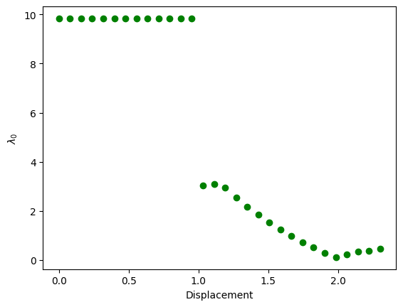
Let’s take a look at the evolution of the first eigenvalue of the reduced Hessian. We can see a sudden reduction in the eigenvalues just after the onset of damage. All eigenvalues are positive, and consequently all states found are stable according to the criteria.

fig = plt.plot(eigenvalues[:, 0], eigenvalues[:, 1], "go", label="Eigenvalues")
plt.xlabel("Displacement")
plt.ylabel(r"$\lambda_0$")

plt.savefig("output/eigenvalues.png")
plt.show()

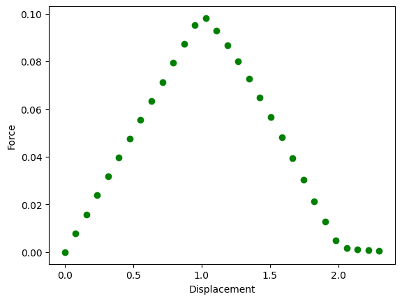
We can also plot also the force displacement diagram and color each point in green if stable or red if unstable.

for i, eigenvalue in enumerate(eigenvalues):
    color = "green" if eigenvalue[1] > 0.0 else "red"
    plt.scatter(ts[i], forces[i], marker="o", color=color)

plt.xlabel("Displacement")
plt.ylabel("Force")

plt.savefig("output/force.png")
plt.show()