Exercise: Implement the LS model from the AT1 state#
Authors:
Jack S. Hale (University of Luxembourg)
Corrado Maurini (Sorbonne Université)
This notebook contains a slightly modified version of the AT1 gradient damage tutorial. Modify it so that it expresses the LS model using the 3rd parameterisation of Table 1 and case b) the intermediate-length bar in Figure 7:
Stability and crack nucleation in variational phase-field models of fracture: effects of length-scales and stress multi-axiality. Zolesi and Maurini 2024. Preprint. https://hal.sorbonne-universite.fr/hal-04552309
Preamble#
We begin by importing the required Python modules.
import sys

from mpi4py import MPI
from petsc4py import PETSc

import matplotlib.pyplot as plt
import numpy as np

import basix
import dolfinx
import dolfinx.fem.petsc
import ufl
from dolfinx import fem, io, mesh, plot

sys.path.append("../utils/")

import pyvista
from evaluate_on_points import evaluate_on_points
from plots import plot_damage_state
Mesh#
We define the mesh using the built-in DOLFINx mesh generation functions for simply geometries.
L = 1.0
H = 0.3
ell_ = 0.1
cell_size = ell_ / 6

nx = int(L / cell_size)
ny = int(H / cell_size)

comm = MPI.COMM_WORLD
msh = mesh.create_rectangle(
    comm, [(0.0, 0.0), (L, H)], [nx, ny], cell_type=mesh.CellType.quadrilateral
)
ndim = msh.geometry.dim

topology, cell_types, geometry = plot.vtk_mesh(msh)
grid = pyvista.UnstructuredGrid(topology, cell_types, geometry)
plotter = pyvista.Plotter()
plotter.add_mesh(grid, show_edges=True, show_scalar_bar=True)
plotter.view_xy()
plotter.add_axes()
plotter.set_scale(5, 5)
if not pyvista.OFF_SCREEN:
    plotter.show()
2026-07-20 14:24:58.935 ( 0.307s) [ 7F6855403140]vtkXOpenGLRenderWindow.:1460 WARN| bad X server connection. DISPLAY=
Setting the stage#
We setup the finite element space, the states, the bound constraints on the states and UFL measures.
We use (vector-valued) linear Lagrange finite elements on quadrilaterals for displacement and damage.
element_u = basix.ufl.element("Lagrange", msh.basix_cell(), degree=1, shape=(msh.geometry.dim,))
V_u = fem.functionspace(msh, element_u)

element_alpha = basix.ufl.element("Lagrange", msh.basix_cell(), degree=1)
V_alpha = fem.functionspace(msh, element_alpha)

# Define the state
u = fem.Function(V_u, name="displacement")
alpha = fem.Function(V_alpha, name="damage")

# Domain measure.
dx = ufl.Measure("dx", domain=msh)
Boundary conditions#
We impose Dirichlet boundary conditions on the displacement and the damage field on the appropriate parts of the boundary.
We do this using predicates. DOLFINx will pass an array of the midpoints of
all facets (edges) as an argument x with shape (3, num_edges) to our
predicate. The predicate we define must return an boolean array of shape
(num_edges) containing True if the edge is on the desired boundary, and
False if not.
def right(x):
    return np.isclose(x[0], L)


def left(x):
    return np.isclose(x[0], 0.0)
The function mesh.locate_entities_boundary calculates the indices of the
edges on the boundary defined by our predicate.
fdim = msh.topology.dim - 1

left_facets = mesh.locate_entities_boundary(msh, fdim, left)
right_facets = mesh.locate_entities_boundary(msh, fdim, right)
The function fem.locate_dofs_topological calculates the indices of the
degrees of freedom associated with the edges. This is the information the
assembler will need to apply Dirichlet boundary conditions.
left_boundary_dofs_ux = fem.locate_dofs_topological(V_u.sub(0), fdim, left_facets)
right_boundary_dofs_ux = fem.locate_dofs_topological(V_u.sub(0), fdim, right_facets)
Using fem.Constant will allow us to update the value of the boundary
condition applied in the pseudo-time loop.
u_D = fem.Constant(msh, 0.5)
bc_ux_left = fem.dirichletbc(0.0, left_boundary_dofs_ux, V_u.sub(0))
bc_ux_right = fem.dirichletbc(u_D, right_boundary_dofs_ux, V_u.sub(0))

bcs_u = [
    bc_ux_left,
    bc_ux_right,
]
and similarly for the damage field.
left_boundary_dofs_alpha = fem.locate_dofs_topological(V_alpha, fdim, left_facets)
right_boundary_dofs_alpha = fem.locate_dofs_topological(V_alpha, fdim, right_facets)

bc_alpha_left = fem.dirichletbc(0.0, left_boundary_dofs_alpha, V_alpha)
bc_alpha_right = fem.dirichletbc(0.0, right_boundary_dofs_alpha, V_alpha)

bcs_alpha = [bc_alpha_left, bc_alpha_right]
Variational formulation of the problem#
Constitutive model#
To implement the S-LS you will need to define new parameters and modify the model functions appropriately.
E, nu = (
    fem.Constant(msh, dolfinx.default_scalar_type(100.0)),
    fem.Constant(msh, dolfinx.default_scalar_type(0.3)),
)
Gc = fem.Constant(msh, dolfinx.default_scalar_type(1.0))
ell = fem.Constant(msh, dolfinx.default_scalar_type(ell_))
c_w = fem.Constant(msh, dolfinx.default_scalar_type(8.0 / 3.0))
eps_c = 0.19364936095953816


def w(alpha):
    """Dissipated energy function as a function of the damage"""
    return alpha


def a(alpha, k_ell=1.0e-6):
    """Stiffness modulation as a function of the damage"""
    return (1 - alpha) ** 2 + k_ell


def eps(u):
    """Strain tensor as a function of the displacement"""
    return ufl.sym(ufl.grad(u))


def sigma_0(eps):
    """Stress tensor of the undamaged material as a function of the strain"""
    mu = E / (2.0 * (1.0 + nu))
    lmbda = E * nu / (1.0 - nu**2)
    return 2.0 * mu * eps + lmbda * ufl.tr(eps) * ufl.Identity(ndim)


def sigma(eps, alpha):
    """Stress tensor of the damaged material as a function of the displacement and the damage"""
    return a(alpha) * sigma_0(eps)
Energy functional and its derivatives#
We use the ufl package of FEniCS to define the energy functional. The
residual (first Gateaux derivative of the energy functional) and Jacobian
(second Gateaux derivative of the energy functional) can then be derived
through automatic symbolic differentiation using ufl.derivative.
f = fem.Constant(msh, PETSc.ScalarType((0.0, 0.0)))
elastic_energy = 0.5 * ufl.inner(sigma(eps(u), alpha), eps(u)) * dx
dissipated_energy = (
    Gc / c_w * (w(alpha) / ell + ell * ufl.inner(ufl.grad(alpha), ufl.grad(alpha))) * dx
)
external_work = ufl.inner(f, u) * dx
total_energy = elastic_energy + dissipated_energy - external_work
To block rigid bode modes in a simple but effective way, we add a very weak elastic foundation.
k_springs = fem.Constant(msh, PETSc.ScalarType(1.0e-8))
very_weak_springs_to_block_rigid_body_modes = k_springs * ufl.inner(u, u) * dx
total_energy += very_weak_springs_to_block_rigid_body_modes
Solvers#
Displacement problem#
The displacement problem (\(u\)) at for fixed damage (\(\alpha\)) is a linear problem equivalent to linear elasticity with a spatially varying stiffness. We solve it with a nonlinear solver which always converges in one Newton step. We use automatic differention to get the first derivative of the energy. We use a direct solve to solve the linear system, but you can also set iterative solvers and preconditioners when solving large problem in parallel.
E_u = ufl.derivative(total_energy, u, ufl.TestFunction(V_u))
E_u_u = ufl.derivative(E_u, u, ufl.TrialFunction(V_u))
elastic_problem = dolfinx.fem.petsc.NonlinearProblem(
    E_u, u, J=E_u_u, bcs=bcs_u, petsc_options_prefix="elastic_"
)

# Create Newton solver and solve
solver_u_snes = elastic_problem.solver
solver_u_snes.setType("ksponly")
solver_u_snes.setTolerances(rtol=1.0e-9, max_it=50)
solver_u_snes.getKSP().setType("preonly")
solver_u_snes.getKSP().setTolerances(rtol=1.0e-9)
solver_u_snes.getKSP().getPC().setType("lu")
Damage problem with bound-constraint#
The damage problem (\(\alpha\)) at fixed displacement (\(u\)) is a variational
inequality due to the irreversibility constraint and the bounds on the
damage. We solve it using a specific solver for bound-constrained provided by
PETSc, called SNESVI. To this end we define with a specific syntax a class
defining the problem, and the lower (lb) and upper (ub) bounds.
E_alpha = ufl.derivative(total_energy, alpha, ufl.TestFunction(V_alpha))
E_alpha_alpha = ufl.derivative(E_alpha, alpha, ufl.TrialFunction(V_alpha))
We now set up the PETSc solver using petsc4py, a fully featured Python wrapper around PETSc.
damage_problem = dolfinx.fem.petsc.NonlinearProblem(
    E_alpha, alpha, bcs=bcs_alpha, J=E_alpha_alpha, petsc_options_prefix="damage_"
)

# Create Newton variational inequality solver and solve
solver_alpha_snes = damage_problem.solver
solver_alpha_snes.setType("vinewtonrsls")
solver_alpha_snes.setTolerances(rtol=1.0e-9, max_it=50)
solver_alpha_snes.getKSP().setType("preonly")
solver_alpha_snes.getKSP().setTolerances(rtol=1.0e-9)
solver_alpha_snes.getKSP().getPC().setType("lu")

# Lower bound for the damage field
alpha_lb = fem.Function(V_alpha, name="lower bound")
alpha_lb.x.array[:] = 0.0
# Upper bound for the damage field
alpha_ub = fem.Function(V_alpha, name="upper bound")
alpha_ub.x.array[:] = 1.0
solver_alpha_snes.setVariableBounds(alpha_lb.x.petsc_vec, alpha_ub.x.petsc_vec)
Before continuing we reset the displacement and damage to zero.
alpha.x.array[:] = 0.0
u.x.array[:] = 0.0
The static problem: solution with the alternate minimization algorithm#
We solve the non-linear problem in \((u,\alpha)\) at each pseudo-timestep by a fixed-point algorithm consisting of alternate minimization with respect to \(u\) at fixed \(\alpha\) and then for \(\alpha\) at fixed \(u\) until convergence is achieved.
We now define a function that alternate_minimization that performs the
alternative minimisation algorithm and assesses convergence based on the
\(L^2\) norm of the difference between the damage field at the current iterate
and the previous iterate.
def simple_monitor(u, alpha, iteration, error_L2):
    print(f"Iteration: {iteration}, Error: {error_L2:3.4e}")


def alternate_minimization(u, alpha, atol=1e-8, max_iterations=100, monitor=simple_monitor):
    alpha_old = fem.Function(alpha.function_space)
    alpha_old.x.array[:] = alpha.x.array

    for iteration in range(max_iterations):
        # Solve for displacement
        elastic_problem.solve()
        # This forward scatter is necessary when `solver_u_snes` is of type `ksponly`.
        u.x.scatter_forward()

        # Solve for damage
        damage_problem.solve()

        # Check error and update
        L2_error = ufl.inner(alpha - alpha_old, alpha - alpha_old) * dx
        error_L2 = np.sqrt(comm.allreduce(fem.assemble_scalar(fem.form(L2_error)), op=MPI.SUM))
        alpha_old.x.array[:] = alpha.x.array

        if monitor is not None:
            monitor(u, alpha, iteration, error_L2)

        if error_L2 <= atol:
            return (error_L2, iteration)

    raise RuntimeError(
        f"Could not converge after {max_iterations} iterations, error {error_L2:3.4e}"
    )
Time-stepping: solving a quasi-static problem#
load_c = eps_c * L  # reference value for the loading (imposed displacement)
loads = np.linspace(0, 1.5 * load_c, 20)

# Array to store results
energies = np.zeros((loads.shape[0], 3))

# File to store the results
file_name = "output/solution.xdmf"
with io.XDMFFile(comm, file_name, "w", encoding=io.XDMFFile.Encoding.HDF5) as file:
    file.write_mesh(msh)

for i_t, t in enumerate(loads):
    u_D.value = t
    energies[i_t, 0] = t

    # Update the lower bound to ensure irreversibility of damage field.
    alpha_lb.x.array[:] = alpha.x.array

    print(f"-- Solving for t = {t:3.2f} --")
    alternate_minimization(u, alpha)
    plot_damage_state(u, alpha)

    # Calculate the energies
    energies[i_t, 1] = comm.allreduce(
        dolfinx.fem.assemble_scalar(dolfinx.fem.form(elastic_energy)),
        op=MPI.SUM,
    )
    energies[i_t, 2] = comm.allreduce(
        dolfinx.fem.assemble_scalar(dolfinx.fem.form(dissipated_energy)),
        op=MPI.SUM,
    )
    with io.XDMFFile(comm, file_name, "a", encoding=io.XDMFFile.Encoding.HDF5) as file:
        file.write_function(u, t)
        file.write_function(alpha, t)
-- Solving for t = 0.00 --
Iteration: 0, Error: 0.0000e+00
-- Solving for t = 0.02 --
Iteration: 0, Error: 0.0000e+00
-- Solving for t = 0.03 --
Iteration: 0, Error: 0.0000e+00
-- Solving for t = 0.05 --
Iteration: 0, Error: 0.0000e+00
-- Solving for t = 0.06 --
Iteration: 0, Error: 0.0000e+00
-- Solving for t = 0.08 --
Iteration: 0, Error: 0.0000e+00
-- Solving for t = 0.09 --
Iteration: 0, Error: 0.0000e+00
-- Solving for t = 0.11 --
Iteration: 0, Error: 0.0000e+00
-- Solving for t = 0.12 --
Iteration: 0, Error: 0.0000e+00
-- Solving for t = 0.14 --
Iteration: 0, Error: 0.0000e+00
-- Solving for t = 0.15 --
Iteration: 0, Error: 0.0000e+00
-- Solving for t = 0.17 --
Iteration: 0, Error: 0.0000e+00
-- Solving for t = 0.18 --
Iteration: 0, Error: 0.0000e+00
-- Solving for t = 0.20 --
Iteration: 0, Error: 2.1272e-02
Iteration: 1, Error: 1.0519e-02
Iteration: 2, Error: 1.4078e-02
Iteration: 3, Error: 2.0070e-02
Iteration: 4, Error: 2.6720e-02
Iteration: 5, Error: 3.3630e-02
Iteration: 6, Error: 3.8487e-02
Iteration: 7, Error: 3.6490e-02
Iteration: 8, Error: 2.6996e-02
Iteration: 9, Error: 2.8528e-02
Iteration: 10, Error: 2.4109e-02
Iteration: 11, Error: 2.8169e-03
Iteration: 12, Error: 5.5855e-05
Iteration: 13, Error: 7.0199e-06
Iteration: 14, Error: 8.2771e-07
Iteration: 15, Error: 2.0786e-07
Iteration: 16, Error: 5.9001e-07
Iteration: 17, Error: 1.8848e-06
Iteration: 18, Error: 6.0223e-06
Iteration: 19, Error: 1.9242e-05
Iteration: 20, Error: 6.1488e-05
Iteration: 21, Error: 1.9671e-04
Iteration: 22, Error: 6.3661e-04
Iteration: 23, Error: 2.2715e-03
Iteration: 24, Error: 9.7396e-03
Iteration: 25, Error: 6.9824e-03
Iteration: 26, Error: 6.4586e-05
Iteration: 27, Error: 8.3250e-07
Iteration: 28, Error: 4.3248e-08
Iteration: 29, Error: 2.2361e-09
-- Solving for t = 0.21 --
Iteration: 0, Error: 1.8095e-04
Iteration: 1, Error: 3.1128e-06
Iteration: 2, Error: 1.1882e-07
Iteration: 3, Error: 4.5037e-09
-- Solving for t = 0.23 --
Iteration: 0, Error: 1.4476e-04
Iteration: 1, Error: 1.9031e-06
Iteration: 2, Error: 5.5300e-08
Iteration: 3, Error: 1.6031e-09
-- Solving for t = 0.24 --
Iteration: 0, Error: 1.1779e-04
Iteration: 1, Error: 1.2044e-06
Iteration: 2, Error: 2.7079e-08
Iteration: 3, Error: 6.1082e-10
-- Solving for t = 0.26 --
Iteration: 0, Error: 9.7227e-05
Iteration: 1, Error: 7.8531e-07
Iteration: 2, Error: 1.3858e-08
Iteration: 3, Error: 2.4690e-10
-- Solving for t = 0.28 --
Iteration: 0, Error: 8.1238e-05
Iteration: 1, Error: 5.2589e-07
Iteration: 2, Error: 7.3745e-09
-- Solving for t = 0.29 --
Iteration: 0, Error: 6.8604e-05
Iteration: 1, Error: 3.6080e-07
Iteration: 2, Error: 4.0656e-09
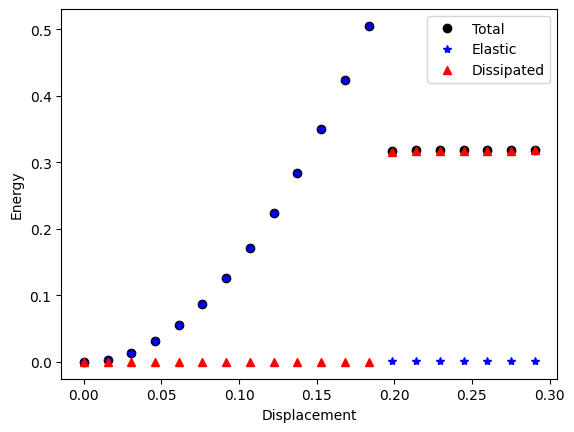
We now plot the total, elastic and dissipated energies throughout the pseudo-time evolution against the applied displacement.
(p3,) = plt.plot(energies[:, 0], energies[:, 1] + energies[:, 2], "ko", linewidth=2, label="Total")
(p1,) = plt.plot(energies[:, 0], energies[:, 1], "b*", linewidth=2, label="Elastic")
(p2,) = plt.plot(energies[:, 0], energies[:, 2], "r^", linewidth=2, label="Dissipated")
plt.legend()

# plt.axvline(x=eps_c * L, color="grey", linestyle="--", linewidth=2)
# plt.axhline(y=H, color="grey", linestyle="--", linewidth=2)

plt.xlabel("Displacement")
plt.ylabel("Energy")

plt.savefig("output/energies.png")
Verification#
The plots above indicates that the crack appears at the elastic limit calculated analytically (see the gridlines) and that the dissipated energy coincides with the length of the crack times the fracture toughness \(G_c\). Let’s check the dissipated energy explicity.
surface_energy_value = comm.allreduce(
    dolfinx.fem.assemble_scalar(dolfinx.fem.form(dissipated_energy)), op=MPI.SUM
)
print(f"The numerical dissipated energy on the crack is {surface_energy_value:.3f}")
print(f"The expected analytical value is {H:.3f}")
The numerical dissipated energy on the crack is 0.318
The expected analytical value is 0.300
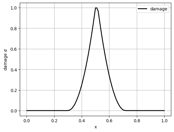
Let’s take a look at the damage profile and verify that we acheive the expected solution for the AT1 model. We can easily see that the solution is bounded between \(0\) and \(1\) and that the decay to zero of the damage profile happens around the theoretical half-width \(D\).
tol = 0.001  # Avoid hitting the boundary of the mesh
num_points = 101
points = np.zeros((num_points, 3))

y = np.linspace(0.0 + tol, L - tol, num=num_points)
points[:, 0] = y
points[:, 1] = H / 2.0

fig = plt.figure()
points_on_proc, alpha_val = evaluate_on_points(alpha, points)
plt.plot(points_on_proc[:, 0], alpha_val, "k", linewidth=2, label="damage")
# plt.axvline(x=0.5 - D, color="grey", linestyle="--", linewidth=2)
# plt.axvline(x=0.5 + D, color="grey", linestyle="--", linewidth=2)
plt.grid(True)
plt.xlabel("x")
plt.ylabel(r"damage $\alpha$")
plt.legend()

# If run in parallel as a Python file, we save a plot per processor
plt.savefig(f"output/damage_line_rank_{MPI.COMM_WORLD.rank:d}.png")