Gradient damage as phase-field models of brittle fracture

Gradient damage as phase-field models of brittle fracture#

Authors:

Jack S. Hale (University of Luxembourg)
Corrado Maurini (Sorbonne Université)

In this notebook we implement a numerical solution of the quasi-static evolution problem for gradient damage models, and show how it can be used to solve brittle fracture problems.

Denote \(u\) the displacement field (vector-valued) and by \(\alpha\) (scalar-valued) the damage field. We consider the energy functional

\[ \mathcal{E}_{\ell}(u, \alpha)= \dfrac{1}{2}\int_{\Omega} a({\alpha}) A_0\,\epsilon(u)\cdot\epsilon(u)\,dx \, + \dfrac{G_c}{c_w} \int_{\Omega}\left( \dfrac{w(\alpha)}{\ell}+ {\ell}\,\nabla {\alpha}\cdot\nabla{\alpha}\right)dx, \]

where \(\epsilon(u) = \tfrac{1}{2}(\nabla u + (\nabla u)^T)\) is the small strain tensor, \(\sigma_0=A_0\,\epsilon=\lambda \mathrm{tr}\epsilon+2\mu \epsilon\) the stress of the undamaged material, with \(\mu\) and \(\lambda\) the usual Lamé parameters, \(a({\alpha})\) the stiffness modulation function that deteriorates the stiffness according to the damage, \(w(\alpha)\) the energy dissipation for a homogeneous process and \(\ell\) the internal length scale.

In the following we will solve, at each pseudo-time step \(t_i\), the minimization problem

\[ \min\mathcal{E}_{\ell}(u, \alpha),\quad u\in\mathcal{C}_i, \alpha\in \mathcal{D}_i, \]

where \(\mathcal{C}_i\) is the space of kinematically admissible displacements at time \(t_i\) and \(\mathcal{D}_i\) the admissible damage field at \(t_i\) that satisfies the irreversibility condition \(\alpha\geq\alpha_{i-1}\).

Here we will

Discretize the problem using (vector-valued) linear Lagrange finite elements on quadrilaterals for the displacement and the damage field.
Use alternate minimization to solve the minimization problem at each time step.
Use PETSc solvers to solve the resulting linear problems and enforce the variational inequality at the discrete level.

We will consider the problem of traction of a two-dimensional bar in plane-stress, where the mesh \( \Omega = [0,L] \times [0,H], \) and the problem is displacement controlled by setting the displacement \(u_x=t\) on the right end, and on the left end \(u_x = 0\). On the bottom boundary we set \(u_y = 0\). Damage is set at zero on the left and right ends.

You can find further information about this model in:

Marigo, J.-J., Maurini, C., & Pham, K. (2016). An overview of the modelling of fracture by gradient damage models. Meccanica, 1-22. https://doi.org/10.1007/s11012-016-0538-4

Preamble#

We begin by importing the required Python modules.

The container images built by the FEniCS Project do not have the sympy module so we install it using pip using the Jupyterbook terminal.

You can install sympy in your JupyterLab by opening a Terminal and running:

pip install sympy

import sys

from mpi4py import MPI
from petsc4py import PETSc

import matplotlib.pyplot as plt
import numpy as np

import basix
import dolfinx
import dolfinx.fem.petsc
import ufl
from dolfinx import fem, la, mesh, plot

sys.path.append("../utils/")

import pyvista
import sympy
from evaluate_on_points import evaluate_on_points
from petsc_problems import SNESProblem
from plots import plot_damage_state
from pyvista.utilities.xvfb import start_xvfb

start_xvfb(wait=0.5)

Mesh#

We define the mesh using the built-in DOLFINx mesh generation functions for simply geometries.

L = 1.0
H = 0.3
ell_ = 0.1
cell_size = ell_ / 6

nx = int(L / cell_size)
ny = int(H / cell_size)

comm = MPI.COMM_WORLD
msh = mesh.create_rectangle(
    comm, [(0.0, 0.0), (L, H)], [nx, ny], cell_type=mesh.CellType.quadrilateral
)
ndim = msh.geometry.dim

topology, cell_types, geometry = plot.vtk_mesh(msh)
grid = pyvista.UnstructuredGrid(topology, cell_types, geometry)
plotter = pyvista.Plotter()
plotter.add_mesh(grid, show_edges=True, show_scalar_bar=True)
plotter.view_xy()
plotter.add_axes()
plotter.set_scale(5, 5)
if not pyvista.OFF_SCREEN:
    plotter.show()

Setting the stage#

We setup the finite element space, the states, the bound constraints on the states and UFL measures.

We use (vector-valued) linear Lagrange finite elements on quadrilaterals for displacement and damage.

element_u = basix.ufl.element("Lagrange", msh.basix_cell(), degree=1, shape=(msh.geometry.dim,))
V_u = fem.functionspace(msh, element_u)

element_alpha = basix.ufl.element("Lagrange", msh.basix_cell(), degree=1)
V_alpha = fem.functionspace(msh, element_alpha)

# Define the state for the Jacobian and residual
u = fem.Function(V_u, name="displacement")
alpha = fem.Function(V_alpha, name="damage")

# Domain measure.
dx = ufl.Measure("dx", domain=msh)

Boundary conditions#

We impose Dirichlet boundary conditions on components of the displacement and the damage field on the appropriate parts of the boundary.

We do this using predicates. DOLFINx will pass an array of the midpoints of all facets (edges) as an argument x with shape (3, num_edges) to our predicate. The predicate we define must return an boolean array of shape (num_edges) containing True if the edge is on the desired boundary, and False if not.

def bottom(x):
    return np.isclose(x[1], 0.0)

def top(x):
    return np.isclose(x[1], H)

def right(x):
    return np.isclose(x[0], L)

def left(x):
    return np.isclose(x[0], 0.0)

The function mesh.locate_entities_boundary calculates the indices of the edges on the boundary defined by our predicate.

fdim = msh.topology.dim - 1

left_facets = mesh.locate_entities_boundary(msh, fdim, left)
right_facets = mesh.locate_entities_boundary(msh, fdim, right)
bottom_facets = mesh.locate_entities_boundary(msh, fdim, bottom)

The function fem.locate_dofs_topological calculates the indices of the degrees of freedom associated with the edges. This is the information the assembler will need to apply Dirichlet boundary conditions.

left_boundary_dofs_ux = fem.locate_dofs_topological(V_u.sub(0), fdim, left_facets)
right_boundary_dofs_ux = fem.locate_dofs_topological(V_u.sub(0), fdim, right_facets)
bottom_boundary_dofs_uy = fem.locate_dofs_topological(V_u.sub(1), fdim, bottom_facets)

Using fem.Constant will allow us to update the value of the boundary condition applied in the pseudo-time loop.

u_D = fem.Constant(msh, 0.5)
bc_ux_left = fem.dirichletbc(0.0, left_boundary_dofs_ux, V_u.sub(0))
bc_ux_right = fem.dirichletbc(u_D, right_boundary_dofs_ux, V_u.sub(0))
bc_uy_bottom = fem.dirichletbc(0.0, bottom_boundary_dofs_uy, V_u.sub(1))

bcs_u = [bc_ux_left, bc_ux_right, bc_uy_bottom]

and similarly for the damage field.

left_boundary_dofs_alpha = fem.locate_dofs_topological(V_alpha, fdim, left_facets)
right_boundary_dofs_alpha = fem.locate_dofs_topological(V_alpha, fdim, right_facets)
bc_alpha_left = fem.dirichletbc(0.0, left_boundary_dofs_alpha, V_alpha)
bc_alpha_right = fem.dirichletbc(0.0, right_boundary_dofs_alpha, V_alpha)

bcs_alpha = [bc_alpha_left, bc_alpha_right]

Variational formulation of the problem#

Constitutive model#

We will now define the constitutive model and the related parameters. In turn these will be used to define the energy. The code is sufficiently generic to allow for a wide class of functions \(w\) and \(a\).

Exercise: Show by dimensional analysis that varying \(G_c\) and \(E\) is equivalent to a rescaling of the displacement by a constant factor.

\[ u_0 = \sqrt{\frac{G_c L}{E}} \]

We can then choose these constants freely in the numerical work (e.g. unitary) and simply rescale the displacement to match the material data of a specific brittle material.

The real material parameters (in the sense that they are those that affect the results) are

the Poisson ratio \(\nu\) and
the ratio \(\ell/L\) between internal length \(\ell\) and the msh size \(L\).

E, nu = (
    fem.Constant(msh, dolfinx.default_scalar_type(100.0)),
    fem.Constant(msh, dolfinx.default_scalar_type(0.3)),
)
Gc = fem.Constant(msh, dolfinx.default_scalar_type(1.0))
ell = fem.Constant(msh, dolfinx.default_scalar_type(ell_))


def w(alpha):
    """Dissipated energy function as a function of the damage"""
    return alpha


def a(alpha, k_ell=1.0e-6):
    """Stiffness modulation as a function of the damage"""
    return (1 - alpha) ** 2 + k_ell


def eps(u):
    """Strain tensor as a function of the displacement"""
    return ufl.sym(ufl.grad(u))


def sigma_0(eps):
    """Stress tensor of the undamaged material as a function of the strain"""
    mu = E / (2.0 * (1.0 + nu))
    lmbda = E * nu / (1.0 - nu**2)
    return 2.0 * mu * eps + lmbda * ufl.tr(eps) * ufl.Identity(ndim)


def sigma(eps, alpha):
    """Stress tensor of the damaged material as a function of the displacement and the damage"""
    return a(alpha) * sigma_0(eps)

Exercise:

Show that it is possible to relate the dissipation constant \(w_1\) to the energy dissipated in a smeared representation of a crack through the following relation:

\[ {G_c}={c_w}\,w_1\ell,\qquad c_w = 4\int_0^1\sqrt{w(\alpha)}d\alpha \]

For the function above we get (we perform the integral with sympy).

z = sympy.Symbol("z")
c_w = 4 * sympy.integrate(sympy.sqrt(w(z)), (z, 0, 1))
print(f"c_w = {c_w}")

c_w = 8/3

The half-width \(D\) of the localisation zone is given by:

\[ D = c_{1/w} \ell,\qquad c_{1/w}=\int_0^1 \frac{1}{\sqrt{w(\alpha)}}d\alpha \]

c_1w = sympy.integrate(sympy.sqrt(1 / w(z)), (z, 0, 1))
D = c_1w * ell_
print(f"c_1/w = {c_1w}")
print(f"D = {D}")

c_1/w = 2
D = 0.200000000000000

The elastic limit of the material is:

\[ \sigma_c = \sqrt{w_1\,E_0}\sqrt{\dfrac{2w'(0)}{s'(0)}}= \sqrt{\dfrac{G_cE_0}{\ell c_w}} \sqrt{\dfrac{2w'(0)}{s'(0)}} \]

Hint: Calculate the damage profile and the energy of a localised solution with vanishing stress in a 1d traction problem

tmp = 2 * (sympy.diff(w(z), z) / sympy.diff(1 / a(z), z)).subs({"z": 0})
sigma_c = sympy.sqrt(tmp * Gc.value * E.value / (c_w * ell.value))
print(f"sigma_c = {sigma_c}")

eps_c = float(sigma_c / E.value)
print(f"eps_c = {eps_c}")

sigma_c = 19.3649360959538
eps_c = 0.19364936095953816

Energy functional and its derivatives#

We use the ufl package of FEniCS to define the energy functional. The residual (first Gateaux derivative of the energy functional) and Jacobian (second Gateaux derivative of the energy functional) can then be derived through automatic symbolic differentiation using ufl.derivative.

f = fem.Constant(msh, PETSc.ScalarType((0.0, 0.0)))
elastic_energy = 0.5 * ufl.inner(sigma(eps(u), alpha), eps(u)) * dx
dissipated_energy = (
    Gc / float(c_w) * (w(alpha) / ell + ell * ufl.inner(ufl.grad(alpha), ufl.grad(alpha))) * dx
)
external_work = ufl.inner(f, u) * dx
total_energy = elastic_energy + dissipated_energy - external_work

Solvers#

Displacement problem#

The displacement problem (\(u\)) at for fixed damage (\(\alpha\)) is a linear problem equivalent to linear elasticity with a spatially varying stiffness. We solve it with a standard linear solver. We use automatic differention to get the first derivative of the energy. We use a direct solve to solve the linear system, but you can also set iterative solvers and preconditioners when solving large problem in parallel.

E_u = ufl.derivative(total_energy, u, ufl.TestFunction(V_u))
E_u_u = ufl.derivative(E_u, u, ufl.TrialFunction(V_u))
elastic_problem = SNESProblem(E_u, u, bcs_u)

b_u = la.create_petsc_vector(V_u.dofmap.index_map, V_u.dofmap.index_map_bs)
J_u = dolfinx.fem.petsc.create_matrix(elastic_problem.a)

# Create Newton solver and solve
solver_u_snes = PETSc.SNES().create()
solver_u_snes.setType("newtonls")
solver_u_snes.setFunction(elastic_problem.F, b_u)
solver_u_snes.setJacobian(elastic_problem.J, J_u)
solver_u_snes.setTolerances(rtol=1.0e-9, max_it=50)
solver_u_snes.getKSP().setType("preonly")
solver_u_snes.getKSP().setTolerances(rtol=1.0e-9)
solver_u_snes.getKSP().getPC().setType("lu")

We test the solution of the elasticity problem

load = 1.0
u_D.value = load

x_u = fem.Function(V_u)
solver_u_snes.solve(None, x_u.x.petsc_vec)

x_alpha = fem.Function(V_alpha)
plot_damage_state(x_u, x_alpha, load=load)

Damage problem with bound-constraint#

The damage problem (\(\alpha\)) at fixed displacement (\(u\)) is a variational inequality due to the irreversibility constraint and the bounds on the damage. We solve it using a specific solver for bound-constrained provided by PETSc, called SNESVI. To this end we define with a specific syntax a class defining the problem, and the lower (lb) and upper (ub) bounds.

E_alpha = ufl.derivative(total_energy, alpha, ufl.TestFunction(V_alpha))
E_alpha_alpha = ufl.derivative(E_alpha, alpha, ufl.TrialFunction(V_alpha))

# We now set up the PETSc solver using petsc4py, a fully featured Python
# wrapper around PETSc.
damage_problem = SNESProblem(E_alpha, alpha, bcs_alpha, J=E_alpha_alpha)

b_alpha = la.create_petsc_vector(V_alpha.dofmap.index_map, V_alpha.dofmap.index_map_bs)
J_alpha = fem.petsc.create_matrix(damage_problem.a)

# Create Newton variational inequality solver and solve
solver_alpha_snes = PETSc.SNES().create()
solver_alpha_snes.setType("vinewtonrsls")
solver_alpha_snes.setFunction(damage_problem.F, b_alpha)
solver_alpha_snes.setJacobian(damage_problem.J, J_alpha)
solver_alpha_snes.setTolerances(rtol=1.0e-9, max_it=50)
solver_alpha_snes.getKSP().setType("preonly")
solver_alpha_snes.getKSP().setTolerances(rtol=1.0e-9)
solver_alpha_snes.getKSP().getPC().setType("lu")

# Lower bound for the damage field
alpha_lb = fem.Function(V_alpha, name="lower bound")
alpha_lb.x.array[:] = 0.0
# Upper bound for the damage field
alpha_ub = fem.Function(V_alpha, name="upper bound")
alpha_ub.x.array[:] = 1.0
solver_alpha_snes.setVariableBounds(alpha_lb.x.petsc_vec, alpha_ub.x.petsc_vec)

Solver description#

A full description of the reduced space active set Newton solver (vinewtonrsls) can be found in:

Benson, S. J., Munson, T. S. (2004). Flexible complimentarity solvers for large-scale applications. Optimization Methods and Software. https://doi.org/10.1080/10556780500065382

We recall the main details here and allow for some mathematical simplifications.

Consider the residual function \(F : \mathbb{R}^n \to \mathbb{R}^n\) and a given a fixed point \(x^k \in \mathbb{R}^n\). Concretely \(F(x^k)\) corresponds to the damage residual vector assembled from the form damage_problem.F and \(x^k\) is the current damage alpha. We now define the active \(\mathcal{A}\) and inactive \(\mathcal{I}\) subsets:

\[ \mathcal{A}(x) := \left\lbrace i \in \left\lbrace 1, \ldots, n \right\rbrace \; | \; x_i = 0 \; \mathrm{and} \; F_i(x) > 0 \right\rbrace \]

\[ \mathcal{I}(x) := \left\lbrace i \in \left\lbrace 1, \ldots, n \right\rbrace \; | \; x_i > 0 \; \mathrm{or} \; F_i(x) \le 0 \right\rbrace \]

For a vector \(F(x^k)\) or matrix \(J(x^k)\) we write its restriction to a set \(\mathcal{I}\) as \(d_{\mathcal{I}}\) and \(J_{\mathcal{I},\mathcal{I}}\), respectively, where the explicit dependence of \(\mathcal{I}\) on \(x\) has been dropped. We define the Newton increment for the current step as \(d = 0\), and set \(d_{\mathcal{A}} = 0\). We then solve the reduced space Newton system for the reduced Newton direction on the inactive set \(d_{\mathcal{I}}\):

\[ [ \nabla F(x^k) ]_{\mathcal{I},\mathcal{I}} d_{\mathcal{I}}^k = -F_{\mathcal{I}}(x^k) \]

Note that by construction the calculated direction is zero on the active set. We then set:

\[ x^{k+1} = \pi[x^k + d^k] \]

where \(\pi\) is the projection onto the variable bounds. This algorithm can be enhanced with a line search procedure to compute how far along the direction \(d^k\) we should move.

Let us now test the solution of the damage problem at a fixed displacement

u.x.array[:] = x_u.x.array
solver_alpha_snes.solve(None, x_alpha.x.petsc_vec)
plot_damage_state(x_u, x_alpha, load=load)

Before continuing we reset the displacement and damage initial guesses to zero.

x_u.x.array[:] = 0.0
x_alpha.x.array[:] = 0.0

The static problem: solution with the alternate minimization algorithm#

We solve the non-linear problem in \((u,\alpha)\) at each pseudo-timestep by a fixed-point algorithm consisting of alternate minimization with respect to \(u\) at fixed \(\alpha\) and then for \(\alpha\) at fixed \(u\) until convergence is achieved.

We now define a function that alternate_minimization that performs the alternative minimisation algorithm and assesses convergence based on the \(L^2\) norm of the difference between the damage field at the current iterate and the previous iterate.

def simple_monitor(u, alpha, iteration, error_L2):
    print(f"Iteration: {iteration}, Error: {error_L2:3.4e}")


alpha_prev = fem.Function(V_alpha)
L2_error = fem.form(ufl.inner(alpha - alpha_prev, alpha - alpha_prev) * dx)


def alternate_minimization(x_u, x_alpha, atol=1e-8, max_iterations=100, monitor=simple_monitor):
    """
    Perform alternate minimisation on displacement and damage problems.

    Args:
        x_u: Initial guess for displacement
        x_alpha: Initial guess for damage
        atol: termination criterion based absolute tolerance as L^2 distance
            between current and previous damage iteration.
        max_iterations: termination criterion on alternate minimisation
            iterations
        monitor: monitor function

    Returns:
        The error and number of iterations.
    """
    for iteration in range(max_iterations):
        # Store previous damage state
        alpha_prev.x.array[:] = x_alpha.x.array

        # Solve for displacement at fixed damage
        alpha.x.array[:] = x_alpha.x.array
        solver_u_snes.solve(None, x_u.x.petsc_vec)

        # Solve for damage at fixed displacement
        u.x.array[:] = x_u.x.array
        solver_alpha_snes.solve(None, x_alpha.x.petsc_vec)

        # Fix damage, check error and update
        alpha.x.array[:] = x_alpha.x.array
        error_L2 = np.sqrt(comm.allreduce(fem.assemble_scalar(L2_error), op=MPI.SUM))

        monitor(x_u, x_alpha, iteration, error_L2)

        if error_L2 < atol:
            return (error_L2, iteration)

    raise RuntimeError(
        f"Could not converge after {max_iterations} iterations, error {error_L2:3.4e}"
    )

Time-stepping: solving a quasi-static problem#

load_c = eps_c * L  # reference value for the loading (imposed displacement)
loads = np.linspace(0, 1.5 * load_c, 20)

# Array to store results
energies = np.zeros((loads.shape[0], 3))

for i_t, t in enumerate(loads):
    u_D.value = t
    energies[i_t, 0] = t

    # Update the lower bound to ensure irreversibility of damage field.
    alpha_lb.x.array[:] = x_alpha.x.array

    print(f"-- Solving for t = {t:3.2f} --")
    error_L2, num_iterations = alternate_minimization(x_u, x_alpha)

    plot_damage_state(x_u, x_alpha)

    u.x.array[:] = x_u.x.array
    alpha.x.array[:] = x_alpha.x.array
    # Calculate the energies
    energies[i_t, 1] = comm.allreduce(
        dolfinx.fem.assemble_scalar(dolfinx.fem.form(elastic_energy)),
        op=MPI.SUM,
    )
    energies[i_t, 2] = comm.allreduce(
        dolfinx.fem.assemble_scalar(dolfinx.fem.form(dissipated_energy)),
        op=MPI.SUM,
    )

-- Solving for t = 0.00 --
Iteration: 0, Error: 0.0000e+00

-- Solving for t = 0.02 --
Iteration: 0, Error: 0.0000e+00
-- Solving for t = 0.03 --
Iteration: 0, Error: 0.0000e+00
-- Solving for t = 0.05 --
Iteration: 0, Error: 0.0000e+00
-- Solving for t = 0.06 --
Iteration: 0, Error: 0.0000e+00
-- Solving for t = 0.08 --
Iteration: 0, Error: 0.0000e+00
-- Solving for t = 0.09 --
Iteration: 0, Error: 0.0000e+00
-- Solving for t = 0.11 --
Iteration: 0, Error: 0.0000e+00
-- Solving for t = 0.12 --
Iteration: 0, Error: 0.0000e+00
-- Solving for t = 0.14 --
Iteration: 0, Error: 0.0000e+00
-- Solving for t = 0.15 --
Iteration: 0, Error: 0.0000e+00

-- Solving for t = 0.17 --
Iteration: 0, Error: 0.0000e+00
-- Solving for t = 0.18 --
Iteration: 0, Error: 0.0000e+00
-- Solving for t = 0.20 --
Iteration: 0, Error: 2.1272e-02
Iteration: 1, Error: 1.0413e-02
Iteration: 2, Error: 1.3875e-02
Iteration: 3, Error: 1.9674e-02
Iteration: 4, Error: 2.6043e-02
Iteration: 5, Error: 3.2666e-02
Iteration: 6, Error: 3.7570e-02
Iteration: 7, Error: 3.6458e-02

Iteration: 8, Error: 2.7801e-02
Iteration: 9, Error: 2.8457e-02
Iteration: 10, Error: 2.5816e-02
Iteration: 11, Error: 4.9179e-03
Iteration: 12, Error: 9.5477e-05
Iteration: 13, Error: 9.4367e-06
Iteration: 14, Error: 1.1155e-06
Iteration: 15, Error: 1.2802e-07
Iteration: 16, Error: 1.4670e-08

Iteration: 17, Error: 1.6981e-09
-- Solving for t = 0.21 --
Iteration: 0, Error: 7.6434e-04
Iteration: 1, Error: 2.8354e-05
Iteration: 2, Error: 2.7208e-06
Iteration: 3, Error: 2.5538e-07
Iteration: 4, Error: 8.1608e-08
Iteration: 5, Error: 2.5724e-07
Iteration: 6, Error: 8.4807e-07
Iteration: 7, Error: 2.7960e-06
Iteration: 8, Error: 9.2182e-06
Iteration: 9, Error: 3.0393e-05
Iteration: 10, Error: 1.0025e-04
Iteration: 11, Error: 3.3226e-04
Iteration: 12, Error: 6.3134e-04
Iteration: 13, Error: 7.8740e-04

Iteration: 14, Error: 5.6695e-04
Iteration: 15, Error: 2.8757e-04
Iteration: 16, Error: 1.0945e-04
Iteration: 17, Error: 3.5396e-05
Iteration: 18, Error: 1.0694e-05
Iteration: 19, Error: 3.1572e-06
Iteration: 20, Error: 9.2565e-07
Iteration: 21, Error: 2.7087e-07
Iteration: 22, Error: 7.9225e-08
Iteration: 23, Error: 2.3172e-08
Iteration: 24, Error: 6.7779e-09
-- Solving for t = 0.23 --
Iteration: 0, Error: 1.5740e-04
Iteration: 1, Error: 3.6150e-05
Iteration: 2, Error: 7.9427e-06
Iteration: 3, Error: 1.7015e-06
Iteration: 4, Error: 3.6252e-07
Iteration: 5, Error: 7.7162e-08

Iteration: 6, Error: 1.6424e-08
Iteration: 7, Error: 3.4964e-09
-- Solving for t = 0.24 --
Iteration: 0, Error: 1.2499e-04
Iteration: 1, Error: 2.1161e-05
Iteration: 2, Error: 3.4709e-06
Iteration: 3, Error: 5.5942e-07
Iteration: 4, Error: 8.9926e-08

Iteration: 5, Error: 1.4453e-08
Iteration: 6, Error: 2.3234e-09
-- Solving for t = 0.26 --
Iteration: 0, Error: 1.0178e-04
Iteration: 1, Error: 1.3134e-05
Iteration: 2, Error: 1.6576e-06
Iteration: 3, Error: 2.0650e-07

Iteration: 4, Error: 2.5691e-08
Iteration: 5, Error: 3.1968e-09
-- Solving for t = 0.28 --
Iteration: 0, Error: 8.4370e-05
Iteration: 1, Error: 8.4968e-06
Iteration: 2, Error: 8.4319e-07
Iteration: 3, Error: 8.2834e-08
Iteration: 4, Error: 8.1322e-09

-- Solving for t = 0.29 --
Iteration: 0, Error: 7.0914e-05
Iteration: 1, Error: 5.6751e-06
Iteration: 2, Error: 4.5039e-07
Iteration: 3, Error: 3.5454e-08
Iteration: 4, Error: 2.7901e-09

We now plot the total, elastic and dissipated energies throughout the pseudo-time evolution against the applied displacement.

(p3,) = plt.plot(energies[:, 0], energies[:, 1] + energies[:, 2], "ko", linewidth=2, label="Total")
(p1,) = plt.plot(energies[:, 0], energies[:, 1], "b*", linewidth=2, label="Elastic")
(p2,) = plt.plot(energies[:, 0], energies[:, 2], "r^", linewidth=2, label="Dissipated")
plt.legend()

plt.axvline(x=eps_c * L, color="grey", linestyle="--", linewidth=2)
plt.axhline(y=H, color="grey", linestyle="--", linewidth=2)

plt.xlabel("Displacement")
plt.ylabel("Energy")

plt.savefig("output/energies.png")

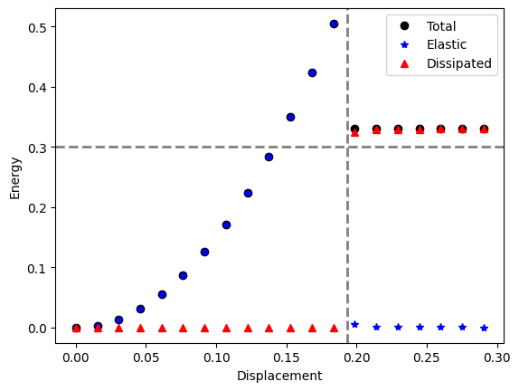
../../_images/43284071a54b8a62c686d6b22204e28558efa12bb97e2b4d9c3af694f25b6263.png

Verification#

The plots above indicates that the crack appears at the elastic limit calculated analytically (see the gridlines) and that the dissipated energy coincides with the length of the crack times the fracture toughness \(G_c\). Let’s check the dissipated energy explicity.

surface_energy_value = comm.allreduce(
    dolfinx.fem.assemble_scalar(dolfinx.fem.form(dissipated_energy)), op=MPI.SUM
)
print(f"The numerical dissipated energy on the crack is {surface_energy_value:.3f}")
print(f"The expected analytical value is {H:.3f}")

The numerical dissipated energy on the crack is 0.330
The expected analytical value is 0.300

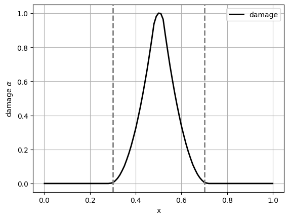
Let’s take a look at the damage profile and verify that we acheive the expected solution for the AT1 model. We can easily see that the solution is bounded between \(0\) and \(1\) and that the decay to zero of the damage profile happens around the theoretical half-width \(D\).

tol = 0.001  # Avoid hitting the boundary of the mesh
num_points = 101
points = np.zeros((num_points, 3))

y = np.linspace(0.0 + tol, L - tol, num=num_points)
points[:, 0] = y
points[:, 1] = H / 2.0

fig = plt.figure()
points_on_proc, alpha_val = evaluate_on_points(alpha, points)
plt.plot(points_on_proc[:, 0], alpha_val, "k", linewidth=2, label="damage")
plt.axvline(x=0.5 - D, color="grey", linestyle="--", linewidth=2)
plt.axvline(x=0.5 + D, color="grey", linestyle="--", linewidth=2)
plt.grid(True)
plt.xlabel("x")
plt.ylabel(r"damage $\alpha$")
plt.legend()

# If run in parallel as a Python file, we save a plot per processor
plt.savefig(f"output/damage_line_rank_{MPI.COMM_WORLD.rank:d}.png")
plt.show()

../../_images/3f1393fc041d92d02cdb8ac286438083e2e67a15abff1271161925af63edac65.png

Exercises#

You can duplicate this notebook by selecting File > Duplicate Python File in the menu. There are many experiments that you can try easily.

Experiment with the regularisation length scale and the mesh size.
Replace the mesh with an unstructured mesh generated with gmsh.
Refactor alternate_minimization as an external function and put it in a seperate .py file and import it into the notebook.
Implement the AT2 model.
Run simulations with:
1. A slab with an hole in the center.
2. A slab with a V-notch.