Linear Elasticity

Linear Elasticity#

Authors:

Laura De Lorenzis (ETH Zürich)
Corrado Maurini (Sorbonne Université)
Jack S. Hale (University of Luxembourg)

This notebook serves as a tutorial to solve a problem of linear elasticity using DOLFINx (the problem solving environment of the FEniCS Project). DOLFINx allows for the concise expression of finite element problems and their efficient parallel solution using the Message Passing Interface (MPI).

You can find a tutorial and useful resources for DOLFINx at the following links

The FEniCS Project Documentation.
The source code, particularly python/tests/unit.
The DOLFINx tutorial,
which includes linear elasticity.

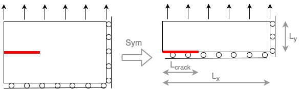
We consider an elastic slab \(\Omega\) with a straight crack \(\Gamma\) subject to a mode I loading by an applied traction force \(f\). Because of symmetry, we can consider only half of the real domain in the computation.

title

We start importing the required libraries.

import sys

from mpi4py import MPI

import numpy as np

import basix
import basix.ufl
import dolfinx.fem as fem
import dolfinx.fem.petsc  # noqa: F401
import dolfinx.io as io
import dolfinx.mesh as mesh
import dolfinx.plot as plot
import ufl

sys.path.append("../utils")
from meshes import generate_mesh_with_crack

Let us generate a mesh using gmsh. The mesh is refined around the crack tip. The function to generate the mesh is implemented in the external file meshes.py located in the directory ../utils. To import it, we add ../utils to the path where the system is looking for possible imports.

Lx = 1.0
Ly = 0.5
Lcrack = 0.3
lc = 0.05
dist_min = 0.1
dist_max = 0.3
comm = MPI.COMM_WORLD
msh, mt, ft, _, _ = generate_mesh_with_crack(
    comm,
    Lcrack=Lcrack,
    Ly=Ly,
    lc=lc,  # characteristic length of the mesh
    refinement_ratio=10,  # how much to refine near the tip zone
    dist_min=dist_min,  # radius of tip zone
    dist_max=dist_max,  # radius of the transition zone
    verbosity=1,
)

To plot the mesh we use pyvista see:

import pyvista  # noqa: E402

pyvista.start_xvfb(wait=0.1)
pyvista.set_jupyter_backend("static")

vtk_mesh = plot.vtk_mesh(msh)
grid = pyvista.UnstructuredGrid(*vtk_mesh)
plotter = pyvista.Plotter()
plotter.add_mesh(grid, show_edges=True)
plotter.camera_position = "xy"
if not pyvista.OFF_SCREEN:
    plotter.show()

Finite element function space#

We use vector-valued linear Lagrange elements on triangles.

element = basix.ufl.element("Lagrange", msh.basix_cell(), degree=1, shape=(msh.geometry.dim,))
V = fem.functionspace(msh, element)

Dirichlet boundary conditions#

We now define the Dirichlet boundary conditions.

In our case we want to

block the vertical component \(u_y\) of the displacement on the part of the bottom boundary without the crack.
block the horizontal component \(u_x\) on the right boundary.

We first get the facets to block on the boundary (dolfinx.mesh.locate_entities_boundary) and then the corresponding dofs (dolfinx.fem.locate_dofs_topological)

def bottom_no_crack(x):
    return np.logical_and(np.isclose(x[1], 0.0), x[0] > Lcrack)


def right(x):
    return np.isclose(x[0], Lx)


# Locate the facets (edges) of the mesh that are on the bottom boundary and not
# on the crack.
bottom_no_crack_facets = mesh.locate_entities_boundary(msh, msh.topology.dim - 1, bottom_no_crack)
# Get the corresponding degrees of freedom.
bottom_no_crack_dofs_y = fem.locate_dofs_topological(
    V.sub(1), msh.topology.dim - 1, bottom_no_crack_facets
)
# And define the Dirichlet boundary condition object.
bc_bottom = fem.dirichletbc(0.0, bottom_no_crack_dofs_y, V.sub(1))

# And same for the right boundary
right_facets = mesh.locate_entities_boundary(msh, msh.topology.dim - 1, right)
right_dofs = fem.locate_dofs_topological(V.sub(0), msh.topology.dim - 1, right_facets)
bc_right = fem.dirichletbc(0.0, right_dofs, V.sub(0))

# Collect the bcs in a list
bcs = [bc_bottom, bc_right]

Define the bulk and surface mesures#

The bulk (dx) and surface (ds) measures are used by ufl to write variational form with integral over the domain or the boundary, respectively.

In this example the surface measure ds includes tags to specify Neumann bcs: ds(1) will mean the integral on the top boundary.

dx = ufl.Measure("dx", domain=msh)
top_facets = mesh.locate_entities_boundary(
    msh, msh.topology.dim - 1, lambda x: np.isclose(x[1], Ly)
)
mt = mesh.meshtags(msh, msh.topology.dim - 1, top_facets, 1)
ds = ufl.Measure("ds", subdomain_data=mt)

Define the variational problem#

We specify the finite element problem to solve using the Unified Form Language syntax by giving the bilinear \(a(u,v)\) and linear forms \(L(v)\) of the weak formulation:

Find the trial function \(u\) such that for all test functions \(v\)

\[ a(u, v) = L(v), \]

with

\[ a(u,v)=\int_{\Omega\setminus\Gamma}\sigma(\varepsilon(u))\cdot \varepsilon(v)\,\mathrm{d}x, \quad L(v)=\int_\Omega b\cdot v \,\mathrm{d}x + \int_{\partial_N\Omega} f\cdot v \,\mathrm{d}s. \]

Note on UFL terminology:

ufl.inner(sigma(eps(u)), eps(v)) is an expression.
ufl.inner(sigma(eps(u)), eps(v)) * dx is a form.

u = ufl.TrialFunction(V)
v = ufl.TestFunction(V)

E = 1.0
nu = 0.3
mu = E / (2.0 * (1.0 + nu))
# Plane strain definition
lmbda = E * nu / ((1.0 + nu) * (1.0 - 2.0 * nu))
# Plane stress definition
lmbda = 2 * mu * lmbda / (lmbda + 2 * mu)


def eps(u):
    """Strain"""
    return ufl.sym(ufl.grad(u))


def sigma(eps):
    """Stress"""
    return 2.0 * mu * eps + lmbda * ufl.tr(eps) * ufl.Identity(2)


def a(u, v):
    """The bilinear form of the weak formulation"""
    return ufl.inner(sigma(eps(u)), eps(v)) * dx


def L(v):
    """The linear form of the weak formulation"""
    # Volume force
    b = fem.Constant(msh, (0.0, 0.0))

    # Surface force on the top
    f = fem.Constant(msh, (0.0, 1.0))
    return ufl.dot(b, v) * dx + ufl.dot(f, v) * ds(1)

Let us plot the solution using pyvista, see

Define the linear problem and solve#

We solve the problem using a direct solver. The class dolfinx.fem.LinearProblem assemble the stiffness matrix and load vector, apply the boundary conditions, and solve the linear system.

problem = fem.petsc.LinearProblem(
    a(u, v), L(v), bcs=bcs, petsc_options={"ksp_type": "preonly", "pc_type": "lu"}
)
uh = problem.solve()
uh.name = "displacement"

Postprocessing#

We can calculate the potential energy.

energy = comm.allreduce(fem.assemble_scalar(fem.form(0.5 * a(uh, uh) - L(uh))), op=MPI.SUM)
print(f"The potential energy is {energy:2.3e}")

The potential energy is -4.139e-01

We can save the results to a file, that can be opened with Paraview.

with io.XDMFFile(MPI.COMM_WORLD, "output/elasticity-demo.xdmf", "w") as file:
    file.write_mesh(uh.function_space.mesh)
    file.write_function(uh)

Stress computation#

We calculate here the Von Mises stress by interpolating the corresponding ufl expression.

sigma_iso = 1.0 / 3.0 * ufl.tr(sigma(eps(uh))) * ufl.Identity(len(uh))
sigma_dev = sigma(eps(uh)) - sigma_iso
von_mises = ufl.sqrt(3.0 / 2.0 * ufl.inner(sigma_dev, sigma_dev))
V_von_mises = fem.functionspace(msh, ("DG", 0))
stress_expr = fem.Expression(von_mises, V_von_mises.element.interpolation_points())
vm_stress = fem.Function(V_von_mises)
vm_stress.interpolate(stress_expr)

from plots import warp_plot_2d  # noqa: E402

plotter = warp_plot_2d(
    uh,
    cell_field=vm_stress,
    field_name="Von Mises stress",
    factor=0.15,
    show_edges=True,
    clim=[0, 2.0],
)

if not pyvista.OFF_SCREEN:
    plotter.show()

with io.XDMFFile(MPI.COMM_WORLD, "output/elasticity-demo.xdmf", "w") as file:
    file.write_mesh(uh.function_space.mesh)
    file.write_function(uh)

We can now wrap all the code in an external module, so that we can re-use the solver later.

We define in elastic_solver.py a function solve_elasticity taking as input the crack length Lcrack, the geoemtric and mesh parameters, the Poisson ratio nu, and giving us as output the solution field uh and the related potential energy energy.

The returned uh and energy will be calculated assuming a force density f=1 on the top surface and a Young modulus E=1. This is without loss of generality, see the exercise below.

Exercise.

Let be \(u^{*}\) and \(P^{*}\) the displacement field obtained on a domain \(\Omega^*=[0,1]\times[0,\varrho]\) for a Young module \(E^*=1\) and a load \(f^*=1\) applied on the top surface. Determine by dimensional analysis the analytical formulas giving the displacement \(u\) and the potential energy \(P\) for any other value of \(E\), load \(f\), and for any domain \(\Omega=[0,L]\times[0,\varrho\, L]\) obtained by a rescaling of \(\Omega^*\) with a length-scale \(L\). Deduce that we can, without loss of generality, perform computation with \(E=1\), \(f=1\) and \(L=1\).